Nowcasting: Maintaining real time estimates of infrequently observed time series
Maintain an estimate of a time series by forecasting the current value using a structural time series model.
Time series analysis appears in every disciple from physiology to retail pricing. A time series variable is typically measured sequentially at fixed intervals of time (often equispaced but not necessarily). Variables may be measured less frequently than theoretically possible for reasons of cost, effort, or convention. With local level linear trend models we can maintain realtime measures of infrequently measured values (see Predicting the Present with Bayesian Structural Time Series). The problem has been referred to as nowcasting because the goal is to maintain a current estimate of the value of a time series by forecasting the current value instead of the future value. The term itself is not very important as the task is essentially a standard forecasting problem.
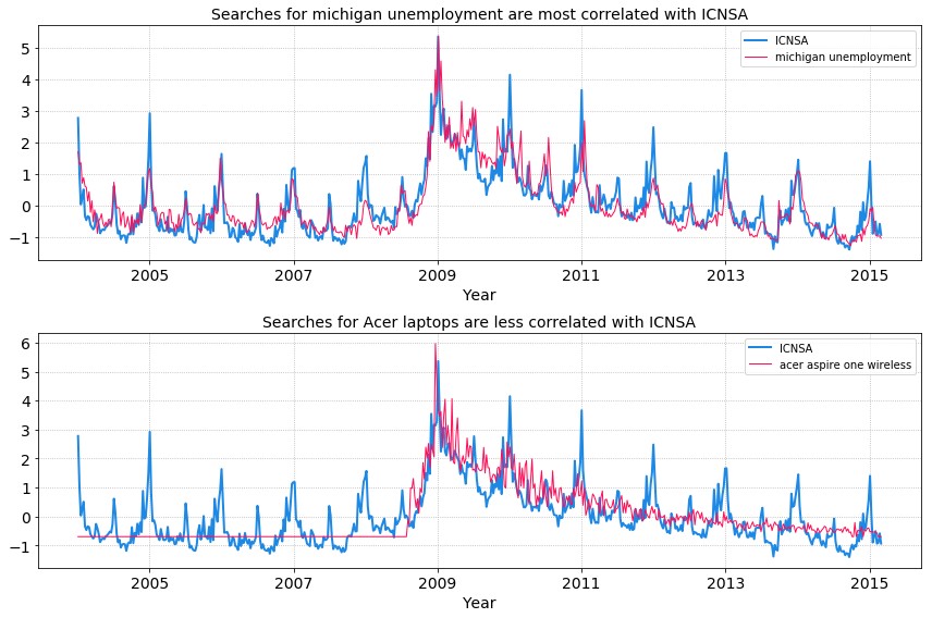
Consider a measurement like US weekly initial claims for unemployment (ICNSA), which is a recession leading indicator. Can we learn this week’s number before it is released? To answer this question we would need a real time signal correlated with the outcome (ICNSA numbers). We can use Google Correlate to extract the top 100 search terms that are most correlated with the ICNSA signal. Google Correlate finds search terms that vary in a similar way to your own time series, ICNSA signal in our case. The 100 search term time series signals are our explanatory (also caled exogenous) variables that can be included as regressors to improve the ICNSA forecast performance. The idea is that contemporaneous signals (exogenous variables) are correlated in time with the unobserved signal (endogenous variable) we are trying to estimate and by regressing on these features can improve our forecast. The temporal structure in these observed signals can be exploited to infer the behaviour of an unobserved signal. Here we will explore using structural time series models that decompose a signal into additive components consisting a linear trend and a mean level.

US weekly initial claims for unemployment (ICNSA)
Brief description of structural time series models
The general approach to time series analysis is to first remove or model the parts that change through time to get a stationary series (a time series is stationary if its statistical properties, like variance, don’t change through time). Next, we use a time series model to capture the correlation in the stationary series. A series can be decomposed into:
- trend components (long-term change in the mean level)
- seasonality component (variation in mean that is periodic in nature and you generally know the period beforehand)
- cycles (variation that oscillates but not according to some known or fixed period)
- exogenous variables that have some correlation with the endogenous variable
- noise
The various components can be combined additively to model the endogenous variable $y$ at time $t$. Such additive models are desirable because we can interpret each term, progressively increase model complexity, and easily diagnose model performance. More concretely a typical model will be written as:
$$ y_t=\mu_t+\gamma_t+\beta^Tx_t+\epsilon_t $$
where $y_t$ is the endogenous variable we want to forecast, $\mu_t$ captures changes in the mean level over time, $\gamma_t$ models the periodic nature of the signal, $\beta^T\boldsymbol{x}_t$ is a regression term with exogenous variables and $\epsilon_t$ is the noise term.
The local linear trend model decomposes the time series into a local level component and a trend component.
$$ \mu_t = \mu_{t-1}+\delta_{t-1}+u_t $$
$$ \delta_t = \delta_{t-1}+v_t $$
The current level of the trend is $\mu_t$, the current “slope” of the trend is $\delta_t$, and the noise terms are $u_t$ and $v_t$.
This kind of model is referred to as UnobservedComponents in statsmodels.
from statsmodels.tsa.statespace.structural import UnobservedComponents

# train on all time points before this and forecast time points after
interventionidx = 200

# df: dataframe with ICNSA and exogenous variables
# regression_columns: exogenous variables
intervention = df.index[interventionidx]
model = UnobservedComponents(
	df.loc[:intervention, 'ICNSA'].values,
	exog = df.loc[:intervention, regression_columns].values,
	level = 'local linear trend'
)
fit = model.fit(maxiter=1000)
We can compare a few models: without exogenous variables from Google Correlate, with the top 10 most correlated search terms, and with the bottom 10 least correlated search terms. The figures below show the ICNSA values in blue and the model predictions in red. The model is trained on observations until 2008 (vertical dashed line) and forecasts are made for the unobserved time after 2008. 95% confidence intervals are in grey.


ICNSA signal with model predictions
It’s clear that adding additional features to the model improves both the fit to the observed data and the forecast. But adding uncorrelated data can have undesired effects on your forecasts. The unobserved components model in statsmodels is unable to pick the best features since it does not have any kind of regularization. Ideally, we want to select only those correlated search terms that gives the best model fit and forecast. The original paper on Bayesian Structural Time Series model provides a methodology for feature selection.
In addition to applications in forecasting, state space models like the one described above can be used to infer the effect of an intervention, like an ad campaign, for counterfactual inference (see Inferring Causal Impact from Bayesian Structural Time-Series Models by Kay Brodersen et. al. (2015))
Useful references: