Time series sequences can be described by their statistical properties like the mean level, trend, perodicity, autocorrelation, variability, and entropy. Most sequence classification models exploit these and other statistical differences between time series signals. However, some features are computationally expensive to calculate and they may not have sufficient discriminative power. Here I will show how Markov chains can be used to derive a simple discriminative statistical measure to separate time series sequences by summarizing the transition probabilities between consecutive timesteps.

A classic paper on ECG time series classification: A new method for detecting atrial fibrillation using R-R intervals by George Moody and Roger Mark (1990), uses markov chains to classify sequences of heart rate measurements as normal sinus rhythm (NS) and atrial fibrillation (AF). By using the sequence of heart rate values directly we don't have to engineer new features and can work with the transition matrix derived from the observed sequence. This method is a good choice when signal variability is informative, as is the case in arrhythmia classification. The method is also computationally inexpensive and easy to deploy on low-power devices. The derived Markov score is also discriminative and can be used as a feature in downstream machine learning models.

The outline of the method is as follows: transitions between consecutive probabilities are summarized in a transition matrix assuming a stationary first-order Markov process (current value depends only on previous value). The log of the ratio of the two transition matrices for group A and group B yields the log-odds matrix \(S\). The score is calculated as the sum of the log-odds for each new observed transition.

In more detail:

• Discretize heart rate into a number of bins. We'll call these bins states.
• Calculate a transition probability (\(p_{i,j}\) = number of transitions from \(state_i\) to \(state_j\) / total number of transitions) between each state and store it in a transition matrix (above figure). We'll call this matrix \(T\). We want a transition matrix for each class. In our example we will be distinguishing a normal sinus rhythm (\(T_\text{NS}\)) from an arrhythmia like atrial fibrilation (\(T_\text{AF}\)).
• Calculate the odds ratio of observing a state transiton in a normal rhythm and an abnormal rhythm: \(p_{i,j}^{\text{NS}} / p_{i,j}^{\text{AF}}\). Store the odds ratios for each state transition in a score matrix \(S\). In practice we can get the score matrix \(S\) simply by dividing the two transition matrices: \(S = T_\text{NS} / T_\text{AF}\).
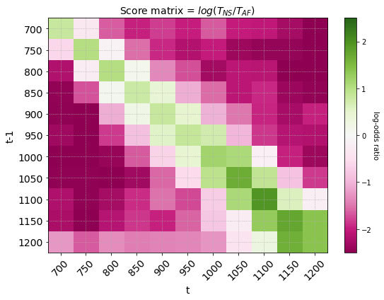
• Take the log of the score matrix so \(S = \text{log}(T_\text{NS} / T_\text{AF})\). This gives us the log odds. We can interpret the score matrix as \(S_{i,j}=0\) if there is an equal likelihood of observing a transition from \(state_i\) to \(state_j\) in both a normal sinus and AF rhythm. Note that taking the \(log(A/B)\) is equivalent to subtracting \(log(A)-log(B)\). It follows that positive values of \(S\) (\(S_{i,j}>0\)) means a greater chance that the state transition from \(state_i\) to \(state_j\) comes from a normal rhythm and negative values of \(S\) (\(S_{i,j}<0\)) means you are more likely to observe the state transition in an AF rhythm.
• To get the final score we sum up the transition probabilities from the score matrix for each observation and choose an appropriate threshold at which we are confident the transition comes from an AF rhythm.

I will use ECG data from the Physionet 2017 Challenge to illustrate how a Markov process is used to classify time series signals. Participants in the challenge had to classify ECG signals collected from mobile sensors as normal sinus rhythm, atrial fibrillation, noise or other. For our purposes we ignore the noise and other labels and simply classify normal and atrial fibrillation.

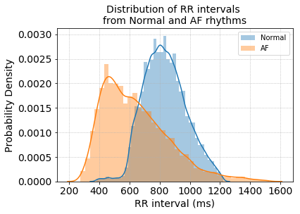
Since the data is provided as raw ECG signals we first extract heart rate by detecting the R-peaks of the ECG beat and calculating the R to R intervals (heart rate = 60 / RR interval in seconds). The distribution of RR intervals between the two groups already shows a good separation between Normal and AF rhythms.

Next, calculate the transition matrix for all RR intervals in the training data.

def transition_matrix(transitions):
    """Takes an array of discrete values and returns a transition matrix
    Args:
        transitions: list of states
    Returns:
        transition matrix, rows must sum to 1
    """
    n = 1 + max(transitions) # number of states
    M = np.zeros((n,n))
    for (i,j) in zip(transitions,transitions[1:]):
        M[i][j] += 1
    # now convert to probabilities:
    for row in M:
        s = sum(row)
        if s > 0:
            row[:] = [f/s for f in row]
    return np.array(M)

The rows of the transition matrix sum to 1 and shows the probability of observing a transition between RR intervals (in milliseconds) from time \(t-1\) to \(t\). The RR intervals were first discretized into bins of step size 50. The coarseness of the discretization is a hyperparameter that can be tuned to find the level that gives the best class separation.

Dividing and taking the log of the two transition matrices gives the us the score matrix where each element is the log-odds ratio of observing a transition between two consecutive states. In the score matrix below, transitions in red are more likely to be observed in atrial fibrilation rhythms and transitions in green are more likely to be observed in normal sinus rhythm.

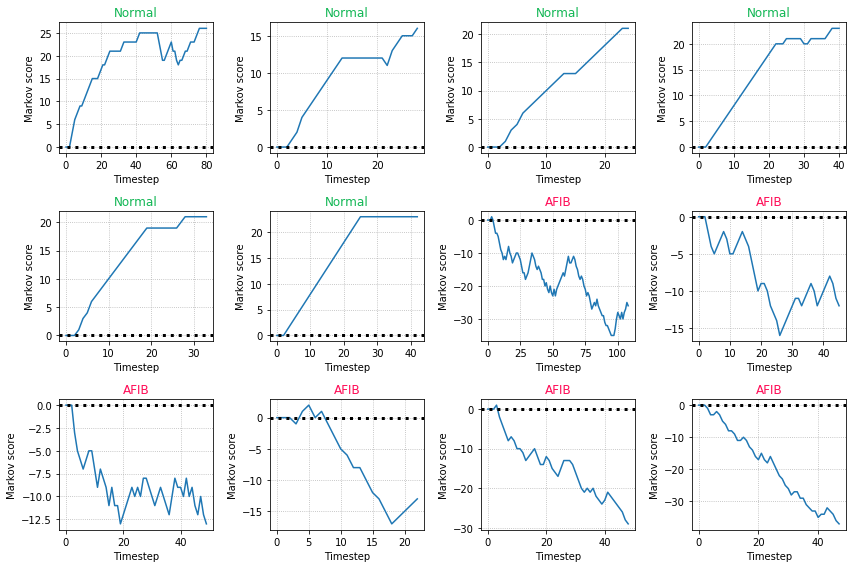
The final score is calculated by summing over transitions in a newly observed sequence of RR intervals.

The score can be plotted over time to show how the score changes with new observations. Examples for normal sinus rhythms have an increasing score and examples with atrial fibrillation have a decreasing score. We can use a cutoff threshold of zero such that a score > 0 will classify the example as a normal sinus rhythm.

Some closing throughts: Why is the Markov score discriminative? Because we calculated the log-odds ratio between the two classes. The score works well in binary classification where the variability between consecutive observations is an informative discriminator. It may not work well in cases where the signal is periodic and the classification accuracy depends on information captured in the periodicity of the signal. In these cases a simple differencing or STL decomposition may help remove the periodic signal. The score presented here is also limited by the fact that it is first-order, meaning we look at only consecutive differences between time \(t-1\) and \(t\). In practice it may be better to use the score as a feature in a machine learning classifier since it captures a discriminiative attribute regarding the variability of the signal.